Dynamic Programming Explained: Solving Dice Roll Probability Problems

When solving problems involving dice roll probabilities, we often need to calculate the number of ways to achieve specific totals. While intuition might tell us that some totals are more likely than others, dynamic programming offers a systematic approach to precisely quantify these probabilities and solve complex counting problems efficiently.

The Dice Roll Probability Problem

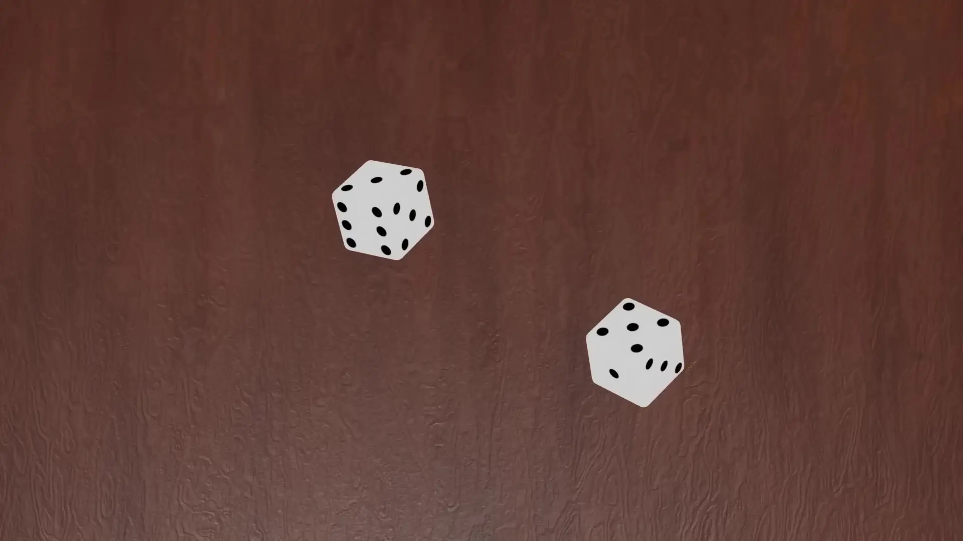
Consider this fundamental question: Given n dice, each with sides numbered 1 through 6, how many different ways can we roll a total of M? For example, with 2 dice, there are 6 ways to roll a sum of 7, but only 1 way to roll a sum of 12. This makes rolling a 7 six times more likely than rolling a 12.

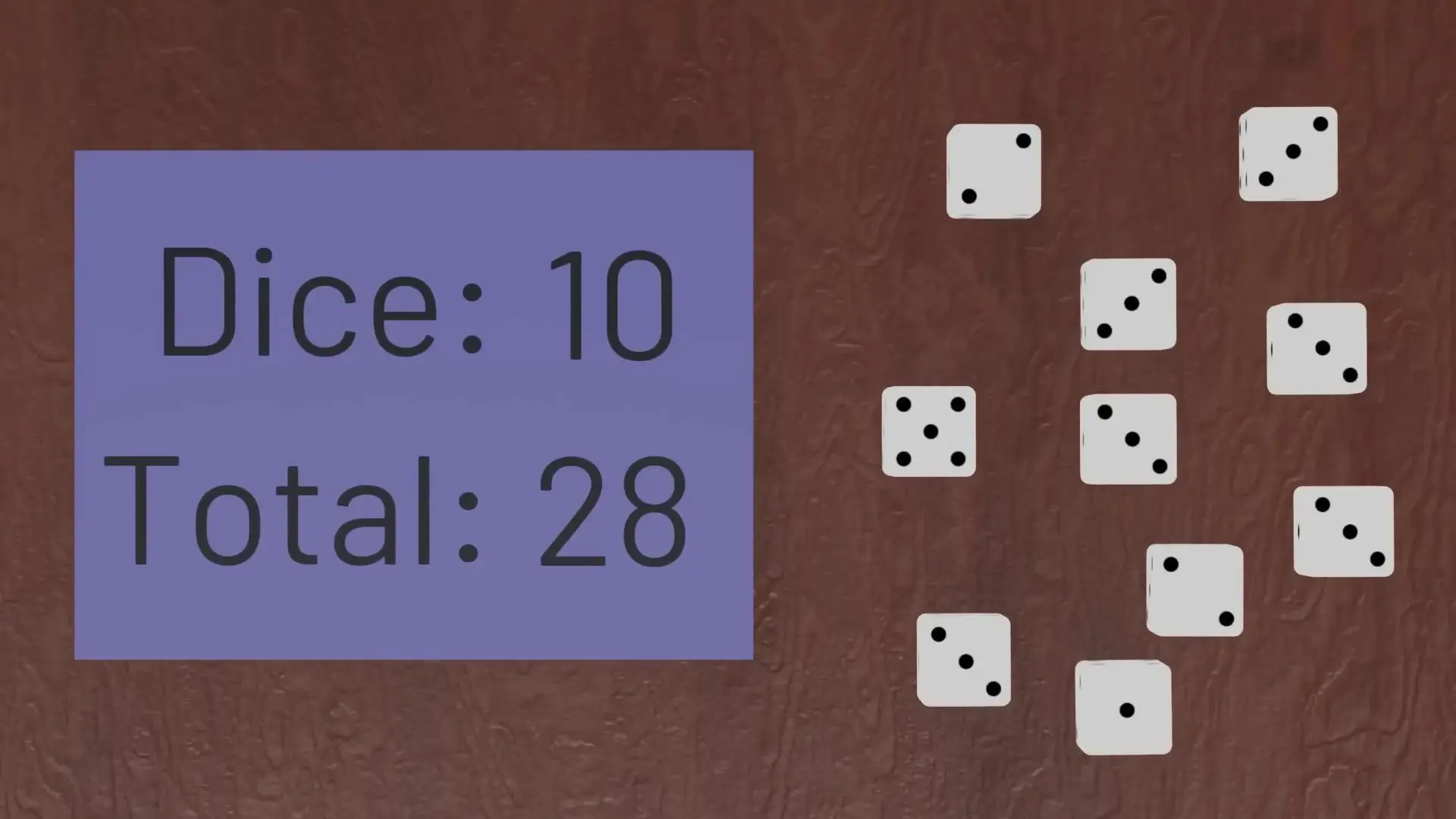
Calculating the probability of specific dice roll totals becomes exponentially complex as the number of dice increases

While calculating these probabilities is straightforward with just two dice, what if we wanted to know how many ways there are to roll a total of 28 with 10 dice? This is where dynamic programming shines as an algorithmic technique.

The Brute Force Approach: Exponential Complexity

The most obvious solution would be to list all possible ways to roll 10 dice and count how many combinations total 28. While correct, this approach quickly becomes impractical. With two dice, we only need to consider 36 possibilities (6² = 36). However, with 10 dice, we'd need to evaluate 6¹⁰ possibilities—more than 60 million combinations!

Even modern computers would struggle with this brute force approach for larger numbers of dice, making it necessary to develop a more efficient algorithm.

Recursive Formulation: Breaking Down the Problem

A key strategy in algorithm design is thinking recursively—solving a big problem by breaking it down into similar smaller problems. For our dice problem, we can formulate it this way: To find the number of ways to roll a total of M with n dice, we need to consider all possible values of the last die (1 through 6) and add up the number of ways to achieve the remaining total with n-1 dice.

Finding a general algorithm for calculating dice roll combinations requires breaking down the problem recursively

Mathematically, this means the number of ways to roll a total of M with n dice equals the sum of the number of ways to roll (M-1), (M-2), (M-3), (M-4), (M-5), and (M-6) with (n-1) dice.

Our base case is simple: with 1 die, there's exactly one way to roll any value from 1 to 6, and zero ways to roll any other value.

The Problem with Pure Recursion: Redundant Calculations

While this recursive formulation is correct, implementing it directly would still be inefficient. The algorithm would repeatedly calculate the same subproblems multiple times, resulting in exponential time complexity similar to the brute force approach.

For example, to calculate the ways to roll 28 with 10 dice, we might need to calculate the ways to roll 24 with 8 dice many times over. This redundancy is where dynamic programming provides its key optimization.

Dynamic Programming Solution: Memoization and Tabulation

The core insight of dynamic programming is to save and reuse the results of subproblems. Instead of recalculating the same values repeatedly, we store them in a lookup table (or memoize them) for future reference.

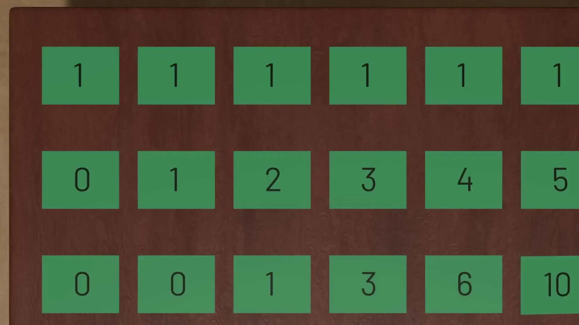
Using a tabulation approach, each cell in our dynamic programming table represents the number of ways to achieve a specific sum with a given number of dice

For our dice problem, we can create a table with n rows (representing the number of dice from 1 to n) and M columns (representing all possible totals from 1 to M). We then fill this table systematically:

Fill the first row (1 die) with 1s for columns 1-6 and 0s elsewhere
For each subsequent row n and column M, calculate the sum of the values in row (n-1) for columns (M-1), (M-2), (M-3), (M-4), (M-5), and (M-6), ignoring negative or zero indices
Continue until the entire table is filled
The value in cell [n][M] gives us our answer

PYTHON

def count_dice_combinations(n_dice, target_sum):
    # Create table with n_dice+1 rows and target_sum+1 columns
    # dp[i][j] represents ways to get sum j with i dice
    dp = [[0 for _ in range(target_sum + 1)] for _ in range(n_dice + 1)]
    
    # Base case: one way to get sum 0 with 0 dice
    dp[0][0] = 1
    
    # Fill the table
    for i in range(1, n_dice + 1):
        for j in range(1, target_sum + 1):
            # Consider all possible values of the current die
            for k in range(1, 7):
                if j - k >= 0:
                    dp[i][j] += dp[i-1][j-k]
    
    return dp[n_dice][target_sum]

This approach dramatically reduces the computational complexity from O(6^n) to O(n×M×6), making it feasible to solve problems with large numbers of dice. For our example of 10 dice and a target sum of 28, we need to fill just a few hundred cells in our table instead of examining millions of combinations.

The Broader Applications of Dynamic Programming

Dynamic programming is not just useful for dice problems; it's a powerful technique applicable to many computational challenges across different domains. The key principles that make it effective are:

Breaking down complex problems into overlapping subproblems
Storing solutions to subproblems to avoid redundant calculations
Building solutions to larger problems from solutions to smaller ones

These principles can be applied to optimization problems, sequence alignment in bioinformatics, resource allocation, scheduling, and many other areas where efficient algorithms are needed to handle exponential complexity.

Conclusion: The Power of Remembering What We've Learned

Dynamic programming embodies a fundamental principle: by remembering what we've already calculated, we can solve complex problems more efficiently. This approach mirrors how humans often solve problems—building on previous knowledge rather than starting from scratch each time.

Whether you're calculating dice probabilities, designing algorithms for machine learning, or solving optimization problems in software development, the principles of dynamic programming provide a powerful framework for tackling computational challenges that would otherwise be intractable.

Dynamic Programming Explained: Solving Complex Dice Roll Probability Problems Efficiently