The Mathematical Origins of Machine Learning: How 19th Century Astronomy Shaped Modern AI

The sophisticated machine learning algorithms powering today's AI systems have their roots in mathematical concepts developed centuries ago. This fascinating connection between historical mathematics and modern technology begins with an astronomical discovery in 1801 that would set the stage for computational approaches we still use today.

The Astronomical Problem That Sparked Mathematical Innovation

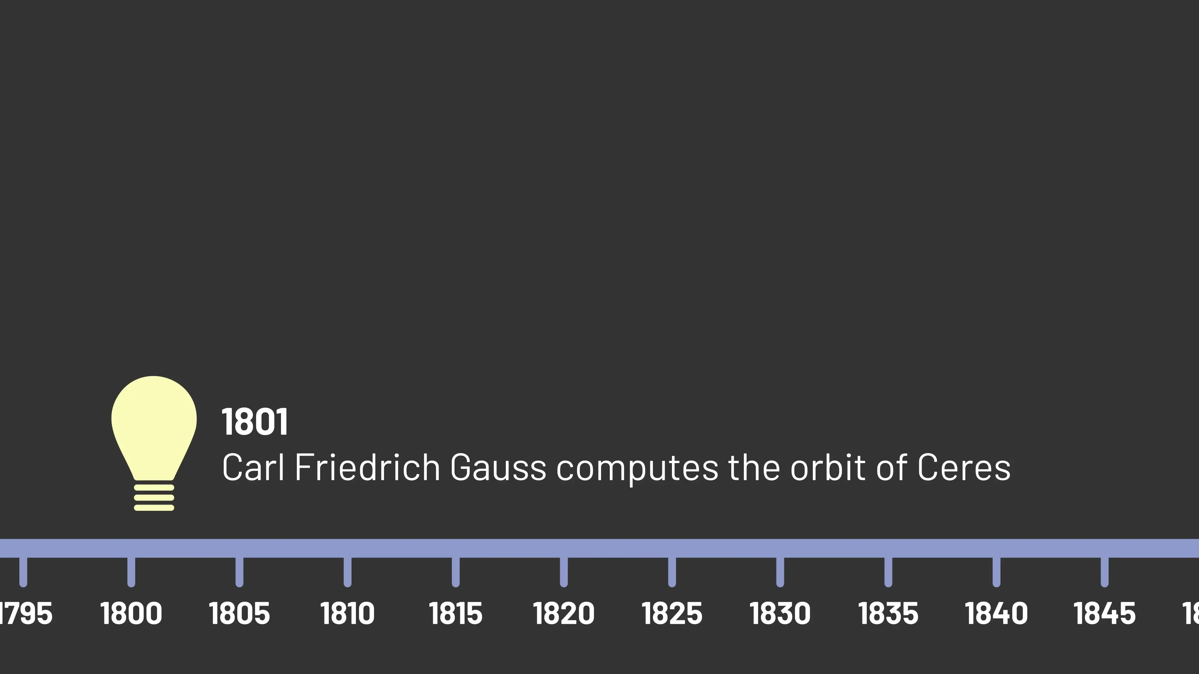
On New Year's Day 1801, Italian astronomer Giuseppe Piazzi observed what he initially thought might be a new star. As he tracked this celestial object over several days, he noticed its position shifted relative to other stars. This was the first sighting of what we now know as Ceres, a dwarf planet located in the asteroid belt between Mars and Jupiter.

Piazzi tracked the planet's position for about a month, carefully recording its location. However, by the time he could alert other astronomers to his discovery, Ceres had moved too close to the sun's glare to remain visible from Earth. The astronomical community faced a critical question: Using just a handful of observations collected over six weeks, could mathematicians calculate Ceres' orbit accurately enough to predict where it would reappear?

This challenge represents the same type of problem that modern machine learning addresses: taking incomplete data, learning the underlying patterns, and using those patterns to make predictions. The mathematical strategies developed to solve this astronomical puzzle would eventually form part of the foundation for today's machine learning techniques.

Least Squares: The Mathematical Method Behind the Solution

A young German mathematician named Carl Friedrich Gauss tackled this problem when others had failed. He understood that a planet's orbit could be defined by several parameters: its size, shape (how circular or elliptical), the tilt of its orbital plane, the rotation of the orbit along that plane, and the planet's position at a given moment.

Gauss developed a strategy that recognized an important reality: Piazzi's measurements weren't perfectly precise. There would inevitably be some error in the observations. This led to a critical question: if no set of parameters could fit the data exactly, which parameters would provide the best fit?

His answer was the method of least squares, a mathematical approach that finds the optimal solution by minimizing the sum of squared differences between observed values and predicted values. To understand this concept, consider a simpler example of linear regression.

Linear Regression and Residuals

When we have a set of data points and want to model the relationship between x and y values with a straight line, we can define that line using two parameters. But which line best fits our data?

For each data point, we can calculate the difference between the actual y-value and what our line predicts. This difference is called the residual. The method of least squares states that the best parameters are those that minimize the sum of squared residuals across all data points.

Why square the residuals? There are several reasons. First, squaring ensures all values are positive, so positive and negative errors don't cancel each other out. Second, squaring more heavily penalizes large errors, which aligns with the statistical reality that smaller errors are more likely than large ones in most measurement systems.

Using this method, Gauss calculated the orbit of Ceres and predicted where it would reappear. In December 1801, astronomers found Ceres exactly where Gauss had predicted, validating his mathematical approach.

From Loss Functions to Gradient Descent

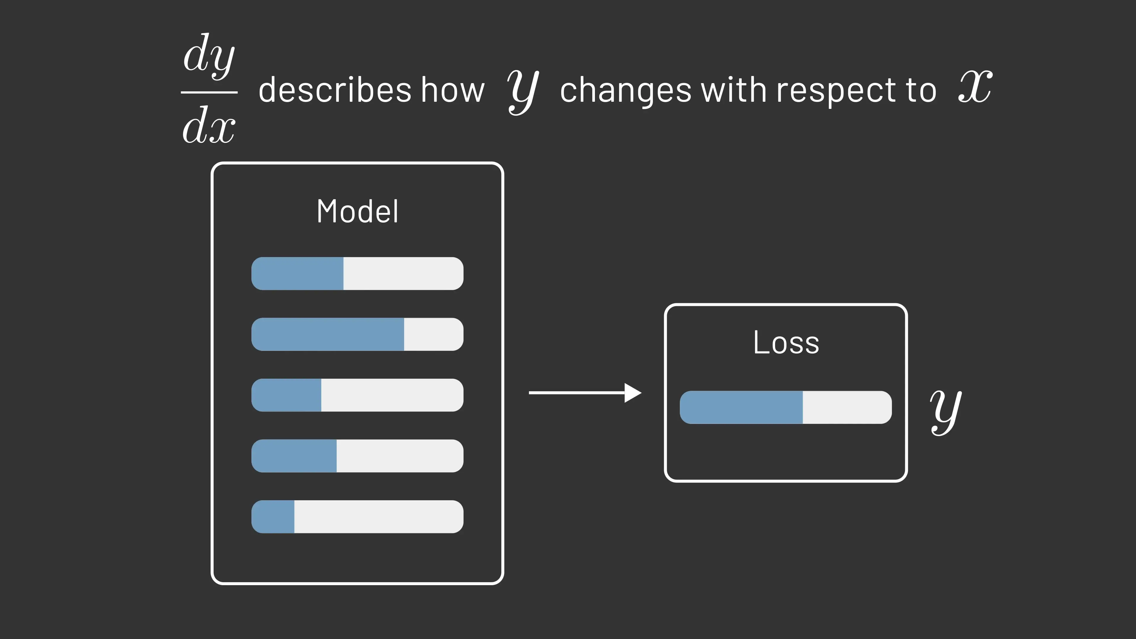
The least squares method represents what we now call a loss function in machine learning. Loss functions measure how far off our predictions are from the actual target values. Our goal in training machine learning models is to learn parameters that minimize the average loss across the dataset.

Modern machine learning models, however, have far more parameters than the six needed for a Kepler orbit. Today's large language models contain billions or even trillions of parameters. To train such complex models efficiently, we need more general strategies for minimizing loss functions.

The Role of Calculus in Machine Learning

This is where calculus, developed by Isaac Newton and Gottfried Wilhelm Leibniz in the 17th century, becomes essential. Calculus studies how changes to the input of a function influence its output. The derivative measures this rate of change.

For functions with multiple inputs (like the multiple parameters in a machine learning model), we use partial derivatives to describe how the output changes when just one input changes. The collection of all partial derivatives for a function is called the gradient, which tells us how changing any parameter will affect the output.

A crucial calculus concept for machine learning is the chain rule, first described by Leibniz in 1676. The chain rule allows us to understand how changes propagate through multiple layers of computation—essential for training neural networks with multiple layers.

Gradient Descent: The Algorithm That Powers Modern Machine Learning

In 1847, French mathematician Augustin-Louis Cauchy described an algorithm now known as gradient descent. This remarkably simple yet powerful approach forms the backbone of most modern machine learning optimization:

1. Start with any set of parameters
2. Compute the gradient, which indicates which direction to move to decrease the function's value
3. Take a small step in that direction
4. Repeat until reaching a minimum

This process allows us to find parameter values that minimize the loss function, resulting in a model that makes more accurate predictions. The elegance of gradient descent is that it works for functions with any number of parameters, making it suitable for today's complex neural networks.

The Mathematical Foundations That Connect Astronomy to AI

The mathematical journey from calculating the orbit of Ceres to training sophisticated neural networks highlights several key concepts that form the mathematical foundations of machine learning:

• Loss functions that measure prediction error (like least squares)
• Optimization techniques to minimize those errors (like gradient descent)
• Calculus principles that enable efficient parameter adjustment (derivatives and the chain rule)
• Statistical approaches that account for noise and uncertainty in data

These mathematical foundations provide the theoretical framework that enables computers to learn from data. While today's machine learning algorithms are far more complex than Gauss's orbital calculations, they build upon the same fundamental principles of using mathematical optimization to find patterns in data.

Conclusion: Mathematics as the Universal Language of Learning

The connection between a 19th-century astronomical calculation and today's cutting-edge AI systems demonstrates how mathematical principles transcend specific applications and time periods. The same mathematical foundations that helped astronomers locate a distant dwarf planet now enable computers to recognize speech, translate languages, and generate creative content.

Understanding these mathematical foundations isn't just of historical interest—it provides deeper insight into how modern machine learning actually works. As we continue to develop more sophisticated AI systems, these fundamental mathematical principles remain at the core of how machines learn from data and make predictions about our world.